autovi: Automated Assessment of Residual Plots Using Computer Vision

useR! 2024

Weihao (Patrick) Li

Monash University

πŸ“Overview

  1. Brief introduction to lineup
  2. Outline of the computer vision model
  3. autovi Package
  4. Shiny app demo

πŸ”Regression Diagnostics

Diagnostics are the key to determining whether there is anything importantly wrong with a regression model.


\[\underbrace{\boldsymbol{e}}_\textrm{Residuals} = \underbrace{\boldsymbol{y}}_\textrm{Observations} - \underbrace{f(\boldsymbol{x})}_\textrm{Fitted values}\]

Graphical approaches (plots) are the recommended methods for diagnosing residuals.

πŸ€”Challenges

  • Vertical spread of the points varies with the fitted values indicates the existence of heteroskedasticity.

  • However, this is an over-interpretation.

  • The visual pattern is caused by a skewed distribution of the predictor.

πŸ”¬Visual Inference

The reading of residual plots can be calibrated by an inferential framework called visual inference (Buja, et al. 2009).

Typically, a lineup of residual plots consists of

  • one actual residual plot
  • \(19\) null plots containing residuals simulated from the fitted model.

To perform a visual test

  • Observer(s) will be asked to select the most different plot(s).
  • The p-value can be calculated using the beta-binomial model (VanderPlas et al., 2021).

🚫Limitations of Lineup Protocol

  1. Human can not
  • evaluate lineup consisted of a large number of plots.
  • evaluate a large number of lineups.
  1. Evaluation of lineup is high in labour cost and time consuming.

πŸ€–Computer Vision Model

Modern computer vision models are well-suited for addressing this challenge.

Source: https://en.wikipedia.org/wiki/Convolutional_neural_network

πŸ“Measure the Difference

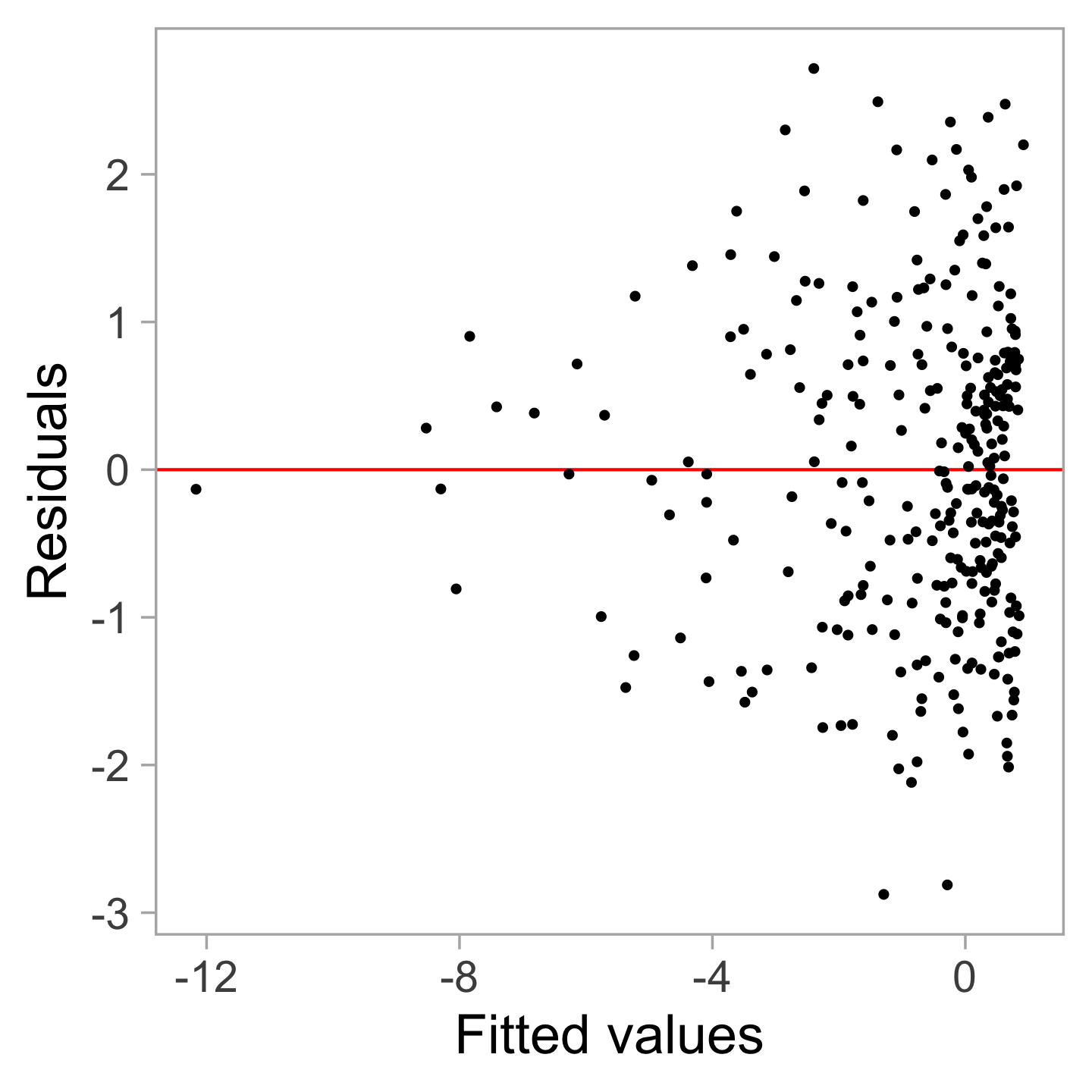
To develop computer vision models assessing lineups of residual plots, we need to define a numerical measure of β€œdifference” or β€œdistance” between plots.

  • pixel-wise sum of square differences
  • Structural Similarity Index Measure (SSIM)
  • scagnostics
  • …

πŸ“KL Divergence of \(P\) from \(Q\)

We defined a distance measure based on Kullback-Leibler divergence to quantify the extent of model violations

\[\begin{align} \label{eq:kl-0} D &= \log\left(1 + \int_{\mathbb{R}^{n}}\log\frac{p(\boldsymbol{e})}{q(\boldsymbol{e})}p(\boldsymbol{e})d\boldsymbol{e}\right), \\ \end{align}\]

  • \(P\): reference residual distribution assumed under correct model specification.

  • \(Q\): actual residual distribution.

  • \(D = 0\) if and only if \(P \equiv Q\).

  • However, \(Q\) is typically unknown \(\Rightarrow\) \(D\) can not be computed.

🎯Estimation of the Distance

We can train a computer vision model to estimate \(D\) with a residual plot

\[\begin{equation} \label{eq:d-approx} \widehat{D} = f_{CV}(V_{h \times w}(\boldsymbol{e}, \boldsymbol{\hat{y}})), \end{equation}\]

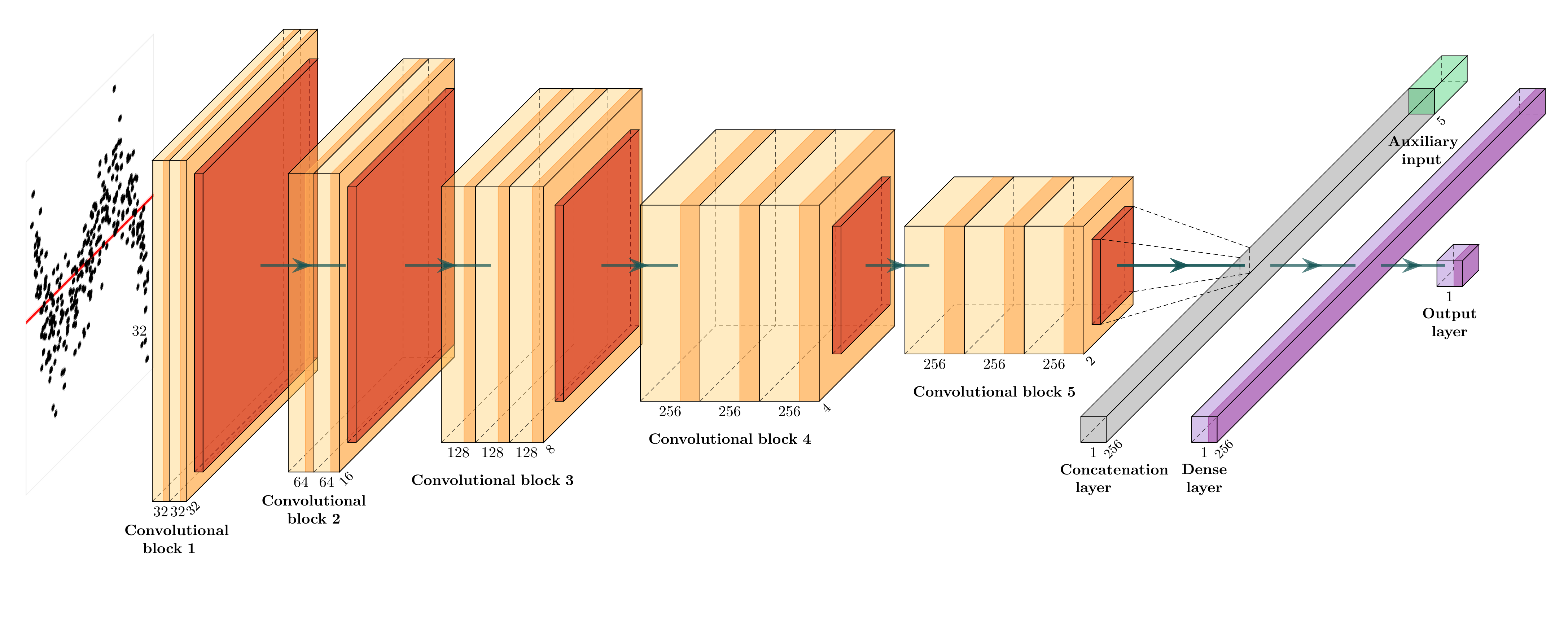
where \(V_{h \times w}(.)\) is a plotting function that saves a residual plot as an image with \(h \times w\) pixels, and \(f_{CV}(.)\) is a computer vision model which predicts distance in \([0, +\infty)\).
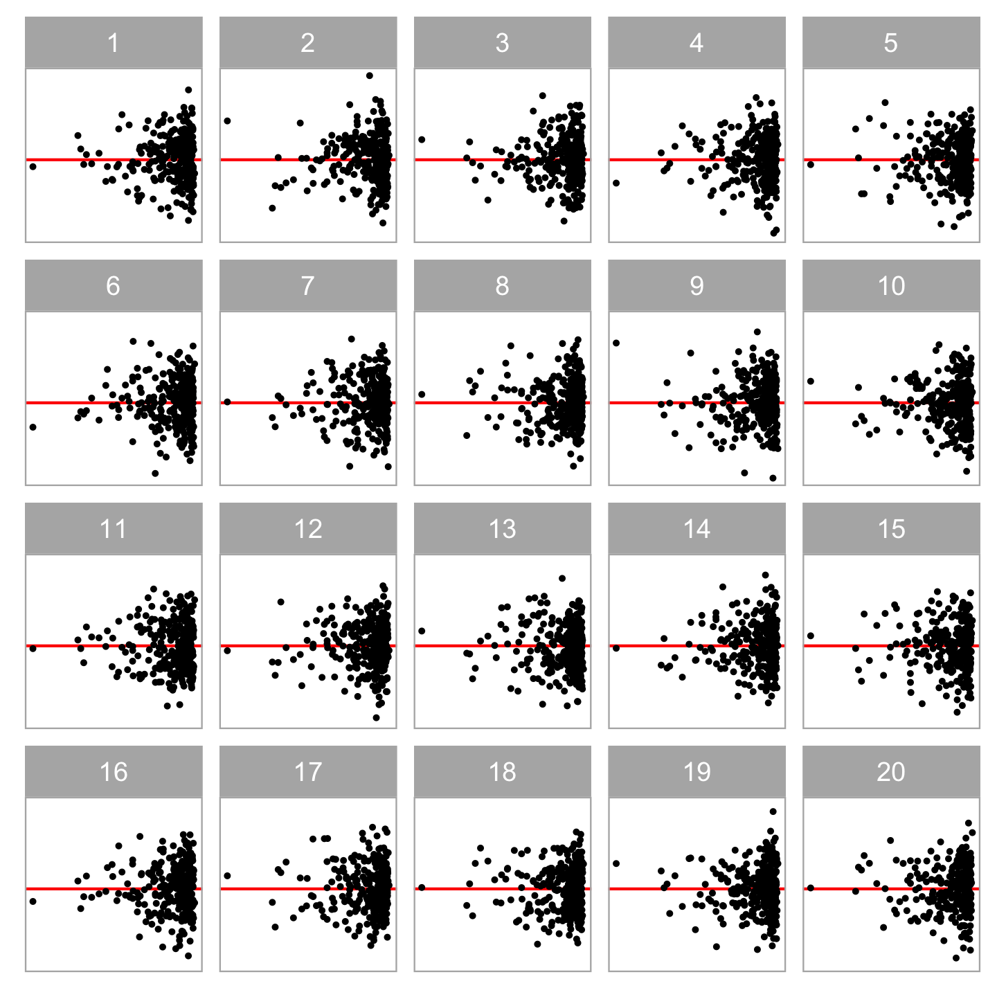
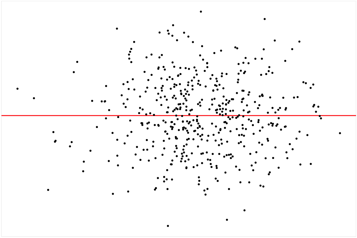
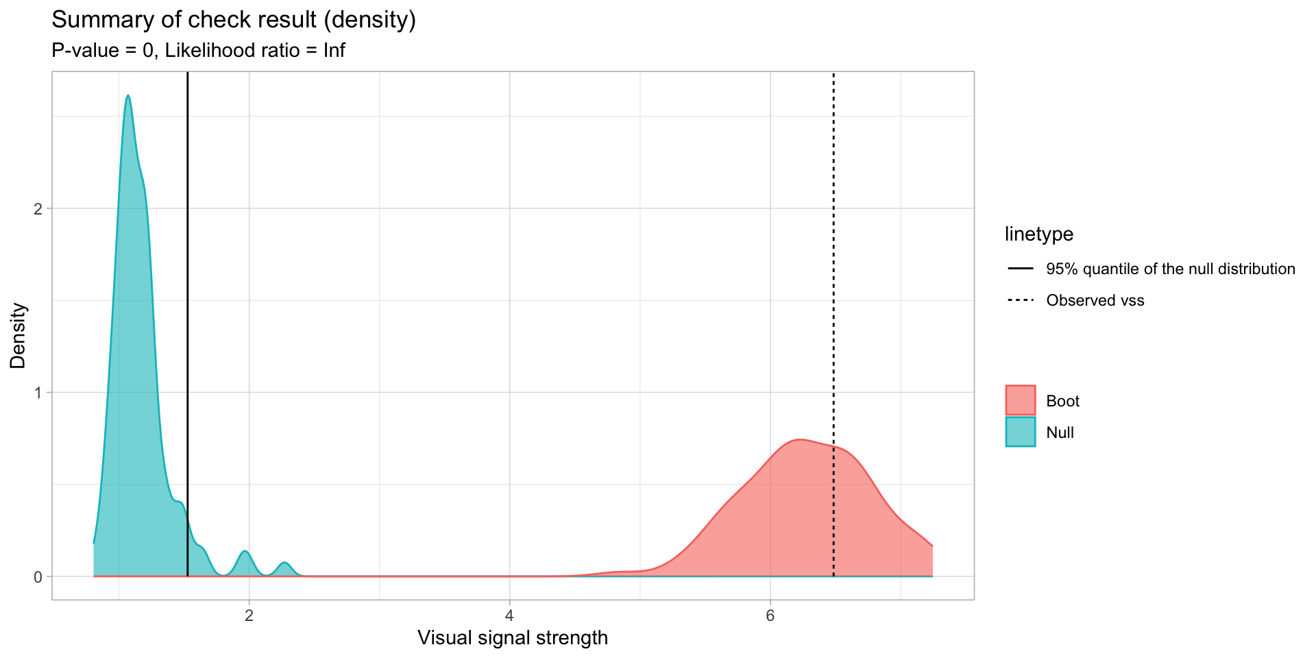
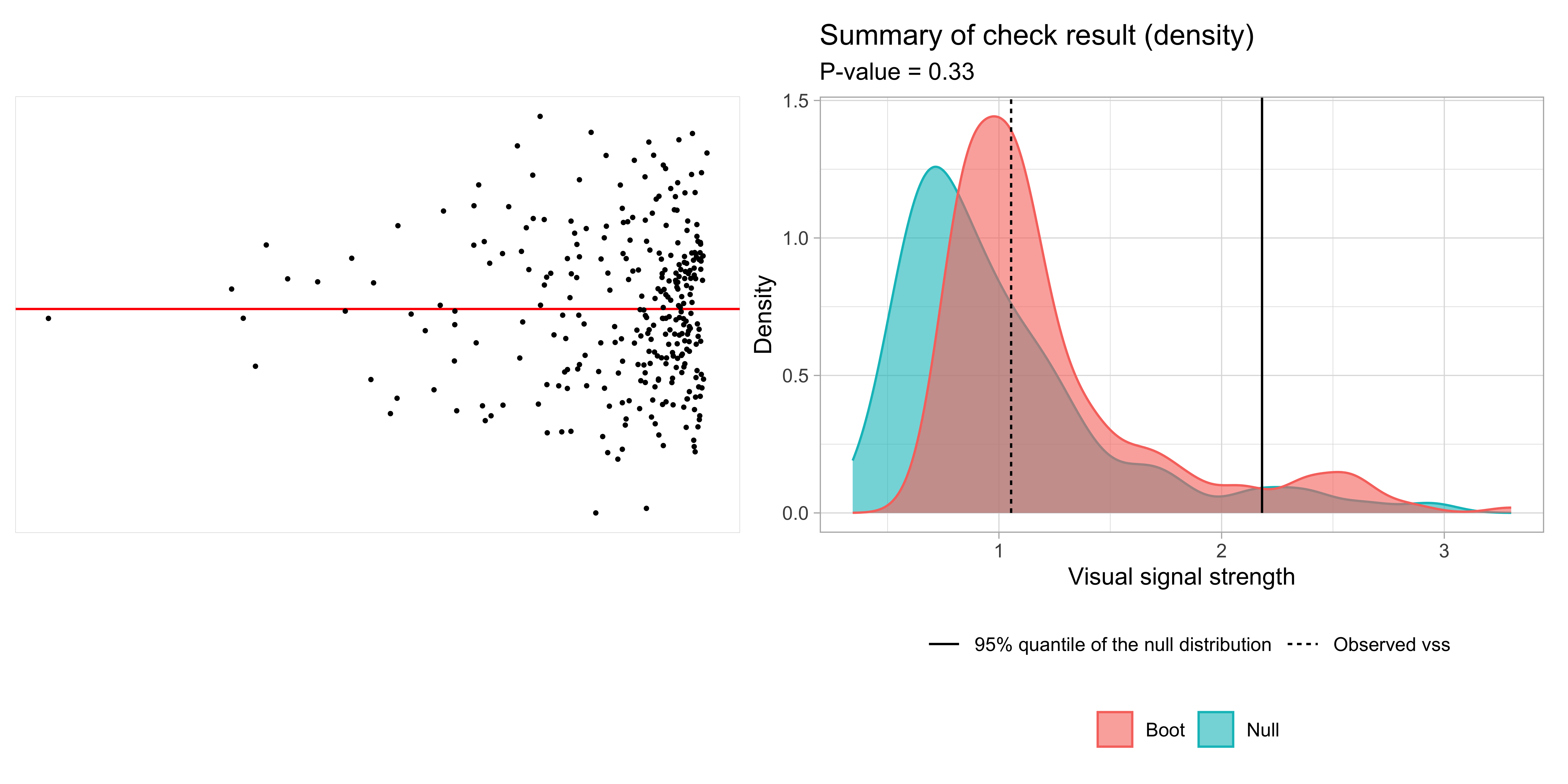
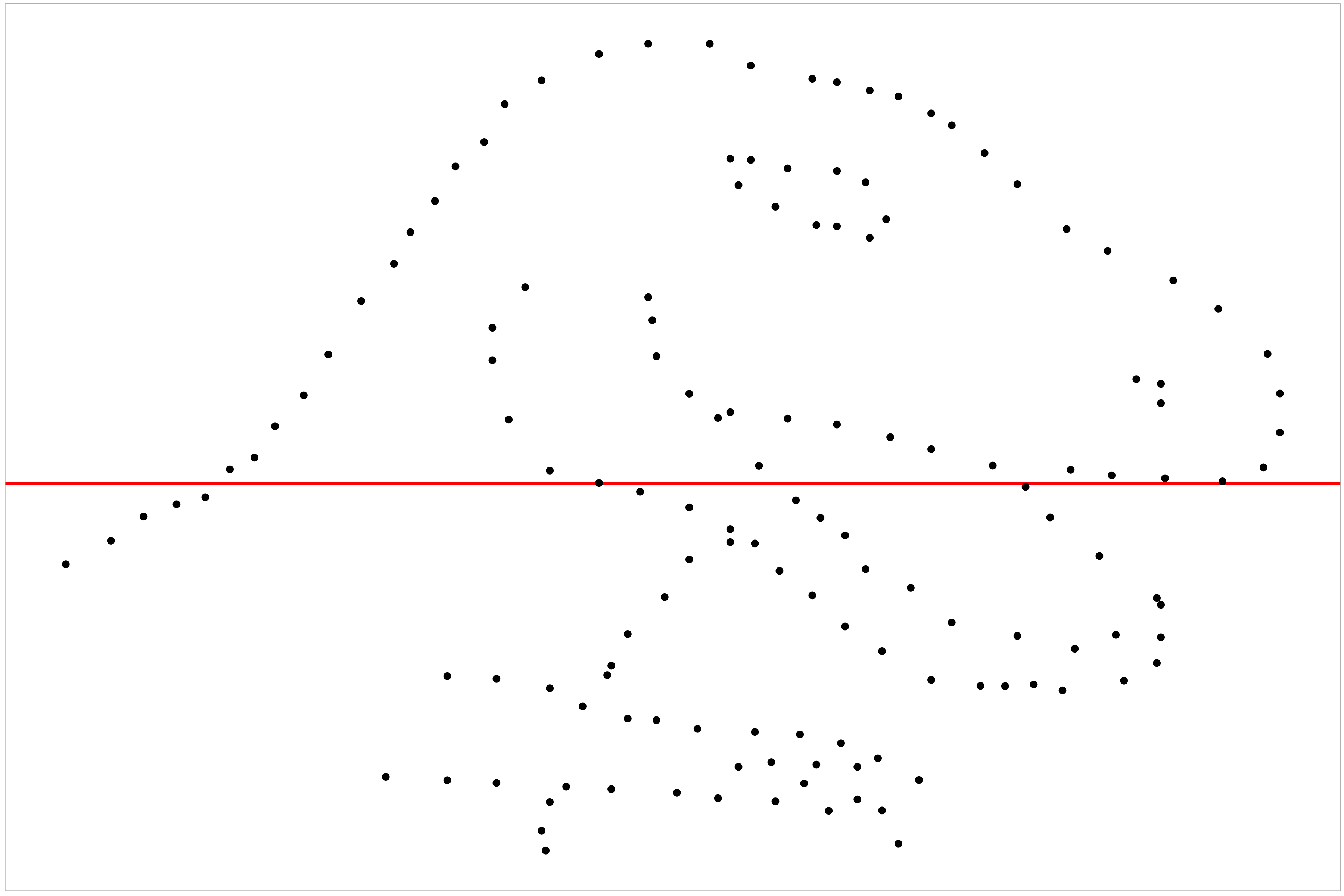
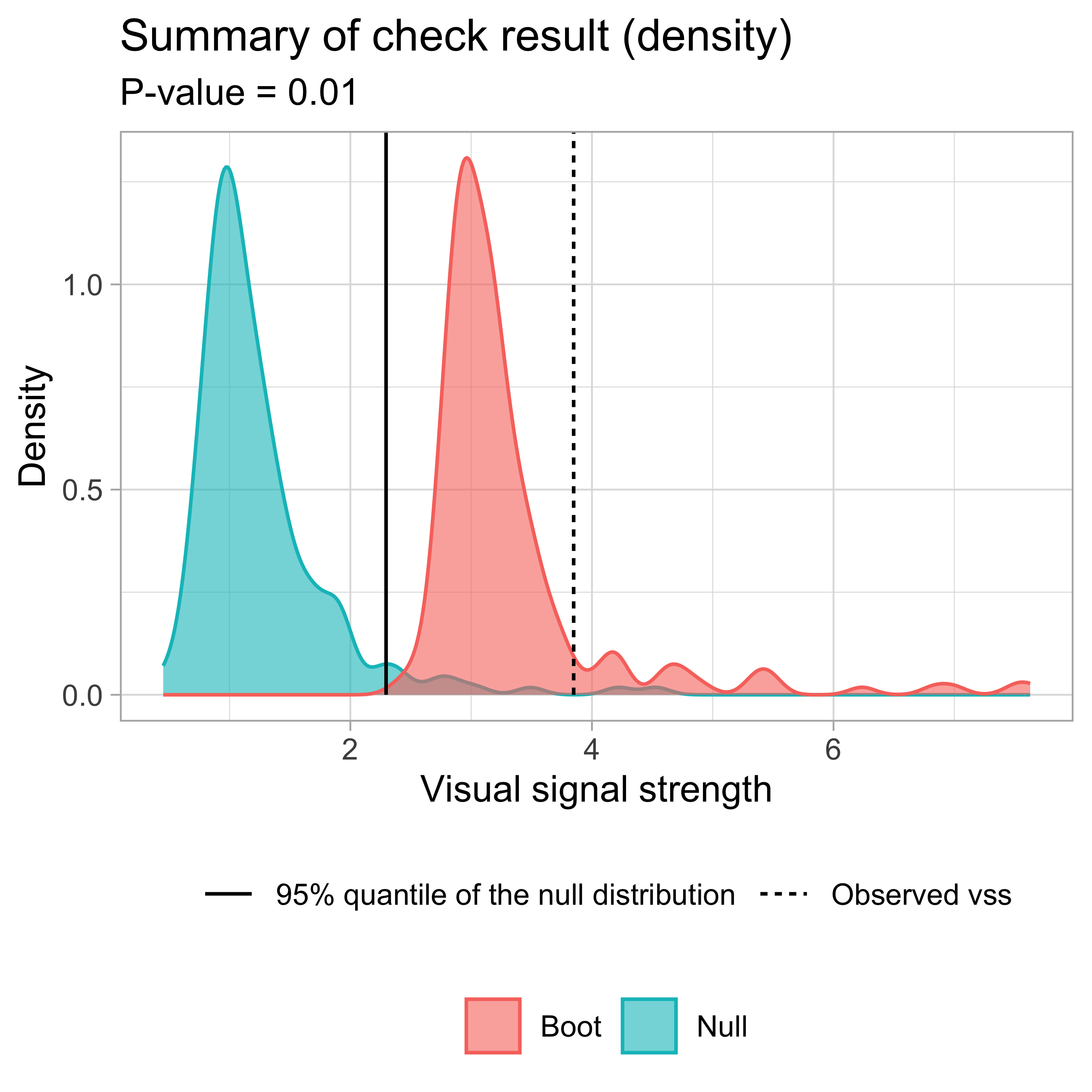
πŸ”¬Statistical Testing

The null distribution can be estimated by predicting \(\widehat{D}\) for a large number of null plots.

  • The critical value can be estimated by the sample quantile (e.g. \(Q_{null}(0.95)\)) of the null distribution.

  • The \(p\)-value is the proportion of null plots having estimated distance greater than or equal to the observed one.
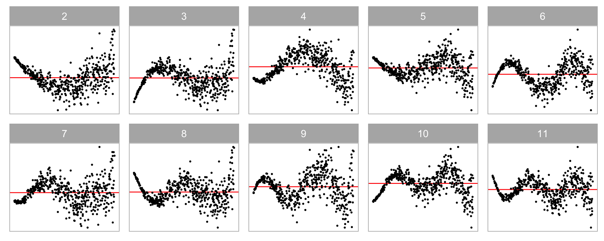
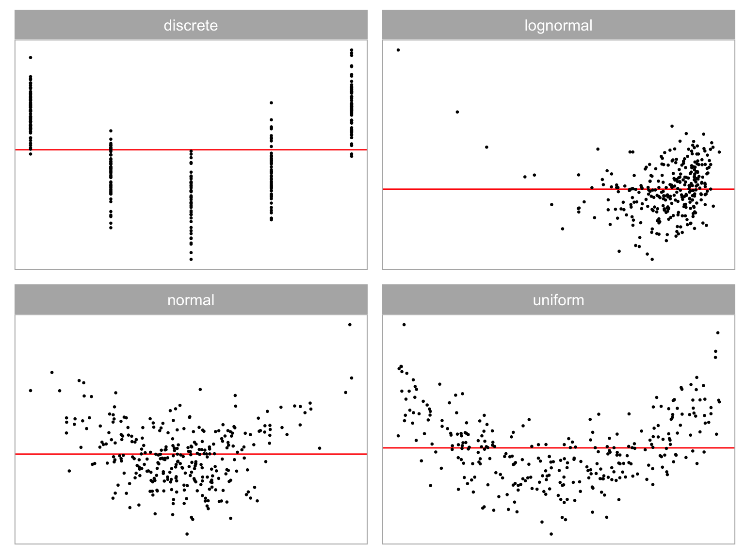
πŸ’‘Training: Various Model Violations

Non-linearity + Heteroskedasticity

Non-normality + Heteroskedasticity
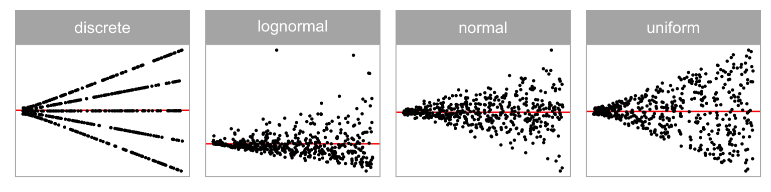
πŸ’‘Training: Predictor Distribution

Distribution of predictor
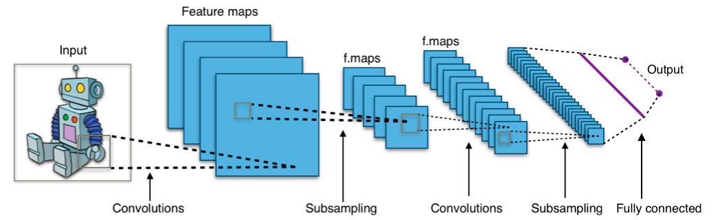
πŸ›οΈModel Architecture

The architecture of the computer vision model is adapted from VGG16 (Simonyan and Zisserman 2014).

autovi Package

The autovi package provides automated visual inference with computer vision models. It is available on CRAN and Github.

Core Methods

  • Null residuals simulation: rotate_resid()
  • Visual signal strength: vss()
  • Comprehensive checks: check() and summary_plot()

πŸ’‘Example: Boston Housing

fitted_model <- lm(MEDV ~ RM + LSTAT + PTRATIO, data = housing)
ggplot() +
  geom_point(aes(fitted(fitted_model), 
                 resid(fitted_model))) +
  theme_void()

rotate_resid()

Null residuals are simulated from the fitted model assuming it is correctly specified.

checker <- auto_vi(fitted_model = fitted_model, 
                   keras_model = get_keras_model("vss_phn_32"))
checker$rotate_resid()
# A tibble: 489 Γ— 2
   .fitted   .resid
     <dbl>    <dbl>
 1 632372.  -33577.
 2 525177.  -82367.
 3 646753. -118729.
 4 624848.  109398.
 5 611817.  -12821.
 6 551051.   -1565.
 7 504757.   54195.
 8 445700.  -70041.
 9 281912.   13595.
10 453398.   64136.
# β„Ή 479 more rows
checker$rotate_resid() |>
  checker$plot_resid()

vss()

Visual signal strength of the actual residual plot

checker$vss()
βœ” Predict visual signal strength for 1 image.
# A tibble: 1 Γ— 1
    vss
  <dbl>
1  6.48

Visual signal strength of a null plot

checker$rotate_resid() |>
  checker$vss()
βœ” Predict visual signal strength for 1 image.
# A tibble: 1 Γ— 1
    vss
  <dbl>
1 0.944

check()

checker$check()
checker
── <AUTO_VI object>
Status:
 - Fitted model: lm
 - Keras model: (None, 32, 32, 3) + (None, 5) -> (None, 1)
    - Output node index: 1
 - Result:
    - Observed visual signal strength: 6.484 (p-value = 0)
    - Null visual signal strength: [100 draws]
       - Mean: 1.169
       - Quantiles: 
          ╔══════════════════════════════════════════╗
          β•‘  25%   50%   75%   80%   90%   95%   99% β•‘
          β•‘1.037 1.120 1.231 1.247 1.421 1.528 1.993 β•‘
          β•šβ•β•β•β•β•β•β•β•β•β•β•β•β•β•β•β•β•β•β•β•β•β•β•β•β•β•β•β•β•β•β•β•β•β•β•β•β•β•β•β•β•β•β•
    - Bootstrapped visual signal strength: [100 draws]
       - Mean: 6.28 (p-value = 0)
       - Quantiles: 
          ╔══════════════════════════════════════════╗
          β•‘  25%   50%   75%   80%   90%   95%   99% β•‘
          β•‘5.960 6.267 6.614 6.693 6.891 7.112 7.217 β•‘
          β•šβ•β•β•β•β•β•β•β•β•β•β•β•β•β•β•β•β•β•β•β•β•β•β•β•β•β•β•β•β•β•β•β•β•β•β•β•β•β•β•β•β•β•β•
    - Likelihood ratio: 0.7064 (boot) / 0 (null) = Extremely large 

summary_plot()

checker$summary_plot()

πŸ’‘Example: Left-triangle

Breusch–Pagan test \(p\)-value = 0.0457

πŸ’‘Example: Dinosaur

Ramsey Regression Equation Specification Error test \(p\)-value = 0.742

Breusch–Pagan test \(p\)-value = 0.36

Shapiro-Wilk test \(p\)-value = 9.21e-05

🌐Shiny Application

Don’t want to install TensorFlow?

Try our shiny web application: https://shorturl.at/DNWzt

🧩Extensions

To diagnose models other than the Classical Normal Linear Regression Model (CNLRM), one can:

  1. Use raw residuals, but be aware that violations may not be identifiable and the test could be two-sided.
  2. Use transformed residuals that are roughly normally distributed.
  3. Reuse the pre-trained convolutional blocks and train a new computer vision model with an appropriate distance measure.

🎬Takeaway

You can use autovi to

  • Evaluate lineups of residual plots of linear regression models

  • Captures the magnitude of model violations through visual signal strength

  • Automatically detect model misspecification using a visual test

Thanks! Any questions?


tengmcing

patrick.li@monash.edu

πŸ“¦ autovi

πŸ“œ Slides